Bluefog Timeline
Bluefog timeline is used to record all activities occurred during your distributed training process. With Bluefog timeline, you can understand the performance of your training algorithm, indentify the bottleneck, and then improve it.
The development of Bluefog timeline is based on the Horovod timeline. Similar to Horovod,
Bluefog timeline clearly visualizes the start and end of all communication stages between
agents such as allreduce, broadcast, neighbor_allreduce, win_put,
win_accumulate and many others. Some of these communication primitives are exclusive
to Bluefog.
An enhanced feature of Bluefog timeline is to visualize the computation states of each
agent such as forward propogation and backward propogation. The visualization of both
communication and computation will help a better understanding of your training algorithm.
For example, Bluefog timeline will tell how your computation is in parallel with the
communication.
Usage
To record a Bluefog timeline, set --timeline-filename command line argument to the
location of the timeline file to be created. This will generate a timeline record file
for each agent. For example, the following command
$ bfrun -np 4 --timeline-filename /path/to/timeline_filename python example.py
will generate four timeline files: timeline_filename0.json, timeline_filename1.json,
timeline_filename2.json, and timeline_filename3.json, and each json file is for
a different agent. You can then load the timeline file into the
chrome://tracing facility of the Chrome browser. If the operation --timeline-filename
is not set, the timeline function will be deactivated by default.
Example I: Logistic regression with neighbor_allreduce
In the first example, we show the timeline when running decentralized SGD for
logistic regression, see the figure below. In this example, each rank is connected
via an undirected power-2 topology. We exploit the
primitive neighbor_allreduce to perform the neighbor averaging.
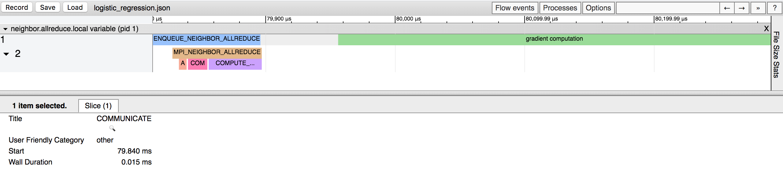
There are two active threads in the timeline: thread 1 that is mainly for gradient
computation and thread 2 for communication. There is a phase MPI_NEIGHBOR_ALLREDUCE
in thread 2 when neighbor allreduce actually happens. It is further divided into multiple
sub-phases:
ALLOCATE_OUTPUT: indicates the time taken to allocate the temporary memory for neighbor’s tensor.COMMUNICATEindicates the time taken to perform the actual communication operation.COMPUTE_AVERAGEindicates the time taken to compuate the average of variables received from neighbors. It is basically a reduce operation.
Another notable feature of this neighbor_allreduce timeline is that threads 1 and 2 are synchronized.
Each time when thread 1 enqueues a task for thread 2 to conduct communication, it will be blocked until
thread 2 finish communication. As a result, it is observed that the end of opeartion ENQUEUE_NEIGHBOR_ALLREDUCE
in thread 1 aligns with the end of opeartion MPI_NEIGHBOR_ALLREDUCE in thread 2.
Example II: Logistic regression with win_accumulate
In this example, we still show the timeline when running decentralized SGD for
logistic regression. Different from Example I, we employ the one-sided communication
primitives win_accumulate to exchange information between neighboring ranks.
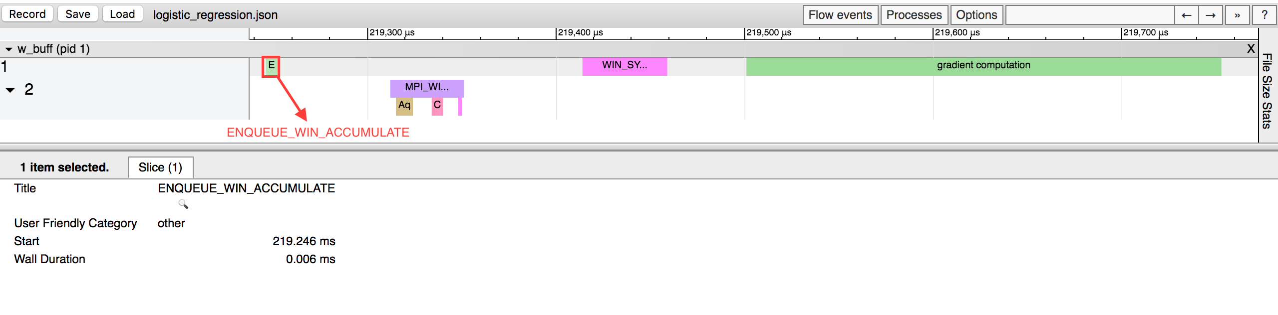
Different from Example I, it is observed that the computation thread (thread 1) and
the communication thread (thread 2) were running independently. Thread 1 will not
be blocked after enqueuing the WIN_ACCUMULATE task to thread 2 (ENQUEUE_WIN_ACCUMULATE in
thread 1 and MPI_WIN_ACCUMULATE in thread 2 are not aligned). In other words,
the one-sided communication primitive enables nonblocking operation and will significantly
improve the training efficiency in real practice.
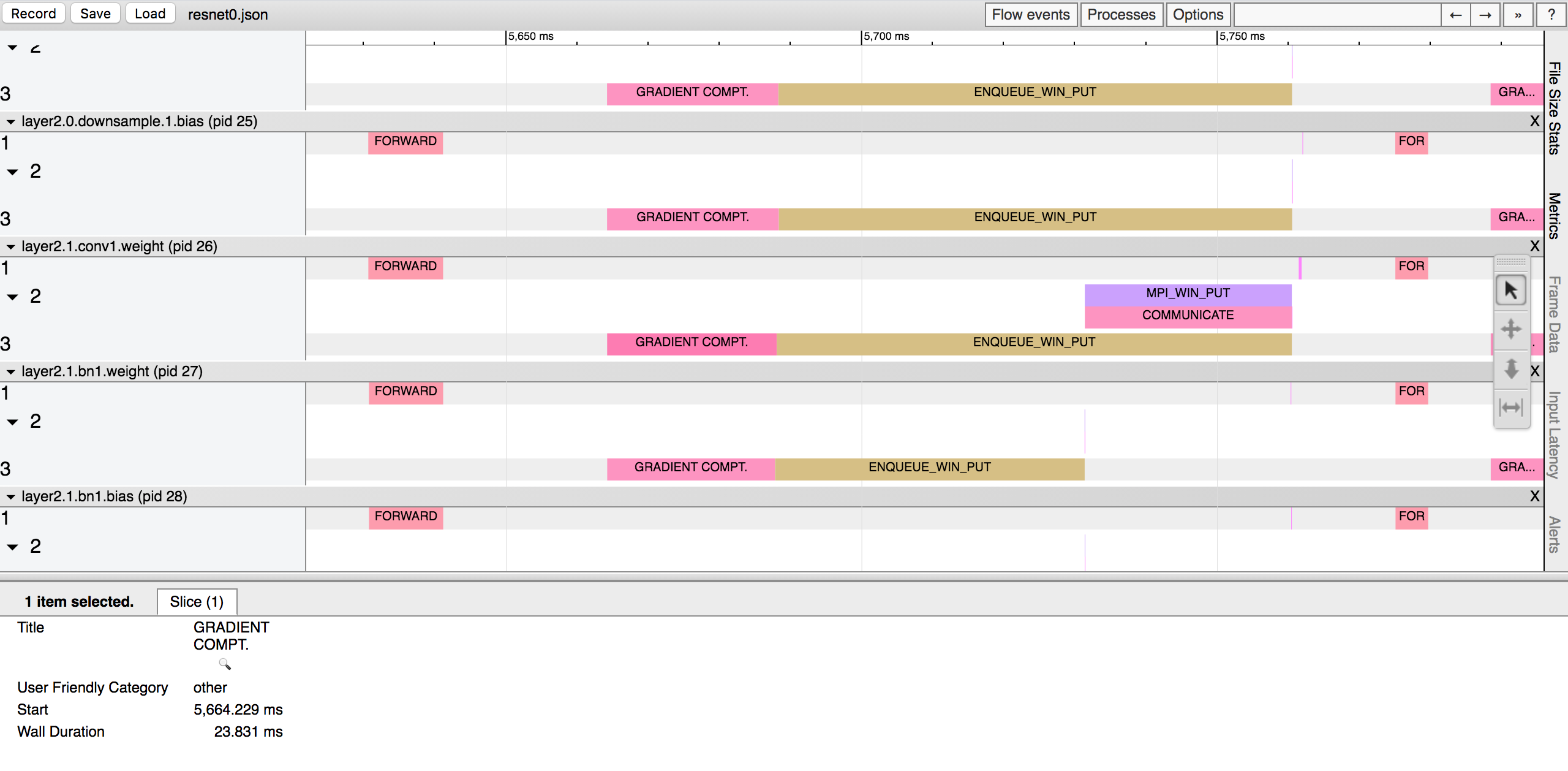
Example III: Resnet training with one-sided communication
In this example, we show the timeline for a real experiment when decentralized SGD is used to
train Resnet with CIFAR10 dataset. We exploit the one-sided communicaton primitive win_put
to exchange information between ranks. It is observed that each phase during the training
is clearly illustrated in the timeline.